Techniques Used by the Certora Prover
In this chapter, we describe some of the techniques used inside the Certora Prover. While this knowledge is not essential for using the Prover, it can sometimes be helpful when the Prover does not behave as expected, for instance in case of a timeout.
Control flow splitting
Note
In addition to the text-form documentation below, there is a brief explanation of control flow splitting in the webinar on timeouts.
Control flow splitting (or “splitting” for short) is one of the techniques that the Certora Prover employs to speed up solving. In the remainder of this section, we will give an overview of how the technique works. This background should be helpful when using the settings described here to prevent Prover timeouts.
Idea
We explain the core idea behind control flow splitting on a simple example.
Whenever there is branching in a program we want to verify, we can look for counterexamples on each branch separately. Basically we split the question A: “Is there a violating execution in the program?” into the two questions B: “Is there a violating execution in the program that takes the first branch?”, and C: “Is there a violating execution in the program that takes the second branch?”. If the answer to either B or C is “yes”, then we can conclude that the answer to A must be “yes”. If the answers to B and C are both “no”, then we can conclude that the answer to A must be “no”.
For example, consider a rule with an if statement:
rule example {
  ...
  if (owner == spender) {
    assert balance_after == balance_before;
  } else {
    assert balance_after == balance_before + amount;
  }
}
To simplify the search for a counterexample, the Prover may internally split this single rule into two rules:
rule example_split_1 {
  ...
  require owner == spender;
  assert balance_after == balance_before;
}

rule example_split_2 {
  ...
  require owner != spender;
  assert balance_after == balance_before + amount;
}
A counterexample for either of the split rules will also be a counterexample for the original rule, and any counterexample for the original rule must violate one of the two split rules, so this splitting doesn’t change the meaning of the rule. However, in some cases the split rule is easier for the Prover to reason about.
Technical Description
On a technical level, splitting is best illustrated using the control flow graph (CFG) of a given CVL rule.
A single splitting step proceeds as follows:
Pick a node with two successors in the CFG, the split point.
Generate two new CFGs, we call them splits; both splits are copies of the original CFG, except that in the first (second) split, the edge to the first (second) successor has been removed. The algorithm also removes all nodes and edges that become unreachable through the removal of the edge.
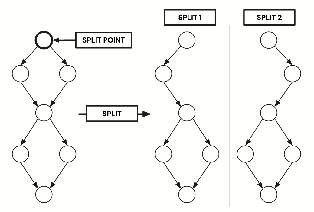
Illustration of a single splitting step
There is an internal heuristic deciding which branching nodes to pick for each single splitting step.
The following pseudo-code illustrates how Certora Prover applies the single splitting in a recursive fashion.
Note
In the remainder of this subsection, we’ll use the terms SAT and
UNSAT. SAT denotes the presence of a counterexample (if the rule
has an assert statement) or a witness example (if the rule has a
satisify statement). UNSAT denotes the absence of any counter- or witness
examples.
Input: input_program_cfg

worklist = []
worklist.add([input_program_cfg, 0])

while (worklist != [])
    [cfg, current_depth] = worklist.pop()

    res = smt_check(cfg, get_timeout_for(current_depth))
    when (res)
        [SAT, model] -> return [SAT, model]
        UNSAT -> continue
        TIMEOUT ->
            if (current_depth == max_depth)
                return timeout
            else
                [split_1, split_2] = split_single(cfg)
                worklist.add([split_1, current_depth + 1])
                worklist.add([split_2, current_depth + 1])
return UNSAT
Intuitively, the algorithm explores the tree of all possible recursive splittings along a fixed sequence of split points up to the maximum splitting depth. We call the splits at maximum splitting depth split leaves. The exploration stops in any of the following three cases:
if one split was found that is SAT (reasoning: if one split is SAT, then the original program must be SAT, since the behavior of the split is replayable in the original program)
if all splits have been shown to be UNSAT
if solving on a split leaf has timed out (except if dontStopAtFirstSplitTimeout has been set)
The settings with which the user can influence this process are the following (each links to a more detailed description of the option):
depth controls the maximum splitting depth.
mediumTimeout controls the timeout that is applied when checking splits that are not split leafs, i.e., that are not at the maximum depth.
smt_timeout controls the timeout that is used to solve split leafs; if this is exceeded, the Prover will give up with a TIMEOUT result, unless the corresponding setting says to go on.
Setting smt_initialSplitDepth to a value above 0 will make the Prover skip the checking and immediately enumerate all splits up to that depth.
Analysis of EVM storage and EVM memory
The Certora Prover works on EVM bytecode as its input. To the bytecode,
the address space of both EVM storage and EVM memory are flat number
lines. That two contract fields x and y don’t share the same memory is an
arithmetic property. With more complex data structures like mappings, arrays,
and structs, this means that every
“non-aliasing” argument
requires reasoning about multiplications, additions, and hash functions.
The Certora Prover models this reasoning correctly, but this naive low-level
modeling can quickly overwhelm SMT solvers. In order to handle storage
efficiently, the Certora Prover analyzes Storage (Memory) accesses in EVM code
in order to understand the Storage (Memory) layout, thus making information like
“an update to mapping x will never overwrite the scalar variable y” much
more obvious to the SMT solvers. For scaling SMT solving to larger programs,
these simplifications are essential.