Timeouts

In the following, we will give a basic classification of timeouts, explain some candidate causes for timeouts, and show ways to sometimes prevent them. See Timeouts in Certora Prover - Theoretical Background for a glimpse into some of the theoretical background on verification timeouts.

Classification of Timeouts

For a first classification of timeouts in Certora Prover, we consider where they occur in the Prover’s pipeline. The pipeline starts by compiling the source code into an intermediate language (called TAC). Many static analyses and program transformations follow this. Afterwards, the TAC program is iteratively split into parts and translated into logical formulas. The logical formulas are then sent to an SMT solver. For more details on how programs are split up, see Control flow splitting. For a more comprehensive overview of the Certora Prover, see the Certora Technology White Paper.

We classify Certora Prover timeouts as follows:

1. timeouts that happen before SMT solvers are running

2. timeouts where the SMT queries in sum lead to a global timeout

3. timeouts where a single SMT query could not be solved

Types 1. and 2. are signified by a hard stop of the Prover. That means the Prover ran into the timeout of the cloud job, which is set at 2 hours, and was forcefully shut down from everything it was doing (it is possible to lower that timeout using the --global_timeout flag). A message like “hard stop reached” appears in the “Global problems” pane of the report, and error symbols next to one or many rules.

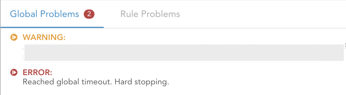
A hard stop message appearing under Global Problems

Type 3. is signified by a soft stop. This means an SMT solver shut down due to hitting the limit for a single SMT run (set via --smt_timeout).

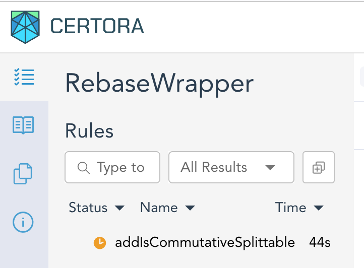
A rule that timed out in the SMT solver

In the remainder, we will focus on the mitigation of SMT timeouts, i.e., types 2. and 3. Non-SMT Timeouts (Type 1.) should be reported to Certora.

Identifying timeout causes

As a first step towards resolving an SMT timeout, we need to diagnose its root causes. In our experience, the following are some of the most common reasons for SMT timeouts:

• non-trivial amount of nonlinear arithmetic

• very high path count

• high Storage/Memory complexity

The term nonlinear arithmetic refers to computations involving multiplications or divisions of variables. These are notoriously hard for solvers. The path count is the number of paths from the initial location to the final location in the rule’s control flow graph. In the worst case, this leads to a very high number of sub-cases that the solver needs to consider. Furthermore, a high number of updates to Storage or Memory can be challenging for the solver, because it needs to reason about aliasing of Storage/Memory locations.

This list is not exhaustive, but the majority of timeouts we have observed so far can be traced back to one or more of these causes. While these are not the only sources of complexity, they provide a good idea of the probable causes for a given timeout.

Complexity feedback from Certora Prover

Certora Prover provides help with diagnosing timeouts. We present these features in this section.

Difficulty statistics

Certora Prover provides statistics on the problem sizes it encounters. These statistics are available in the TAC Reports that are generated in case of an SMT timeout. The statistics are structured according to the timeout reasons given above.

Currently, the Prover tracks the following statistics:

• nonlinear operations count

• path count

• memory/storage complexity measures

For a very short summary we give one summarizing number for each of the statistics, along with a LOW/MEDIUM/HIGH statement.

The meanings of the LOW/MEDIUM/HIGH classifications are as follows:

• LOW: unlikely to be a reason for a timeout

• MEDIUM: might be a reason for a timeout; the timeout might also be a result of the combined complexity with other measures

• HIGH: likely to be a reason for a timeout, even if it is the only aspect of the verification problem that shows high complexity

For more details on the individual statistics and how to make use of them, also see the section on Dealing with different kinds of complexity below.

Timeout TAC reports

A TAC graph for each verification item is linked in the verification report. In case of a timeout, this graph contains information on which parts of the program were part of the actual timeout and which were already solved successfully. It also contains statistics on the timeout causes mentioned above.

In the timeout case, the TAC reports contain additional information that should help diagnose the timeout.

Finding timeout causes through modularization

In addition to the other techniques described here, it can be insightful to remove parts of the code in order to isolate the timeout reason. If timeouts are eliminated through this, modular verification techniques can be employed in order to prove correctness of the parts separately. These techniques are a relatively blunt instrument, but can be necessary in particular with large or complex code bases.

Sanity rules

One way of isolating the timeout cause is by running with a trivial specification. This way, the specification is ruled out as the source of complexity. Thus, a timeout on such a rule hints towards some parts of the program code being challenging for the solver, rather than the program code in combination with another, less trivial, spec.

Sanity rules are such trivial specifications. For documentation on them, see sanity and deep sanity.

Library contracts

Note

This section is EVM-specific and does not apply to Solana or Soroban.

Some systems are based on multiple library contracts that implement business logic. They also forward storage updates to a single external contract holding the storage.

In these systems, it can be appropriate to verify each library independently.

If you encounter timeouts when trying to verify the main entry point contract to the system, check the impact of the libraries on the verification by summarizing all external library (delegate) calls as NONDET, using the option -summarizeExtLibraryCallsAsNonDetPreLinking as follows:

certoraRun ... --prover_args '-summarizeExtLibraryCallsAsNonDetPreLinking true'

Note

This option is only applied to delegatecalls and external library calls. The Solidity compiler automatically inlines internal calls, and they are subject to summarizations specified in the spec file’s methods block.

Timeout prevention

Timeout prevention approaches fall into these categories:

1. Changing prover settings

2. Changing specs

3. Changing source code

Changing Prover settings is the least invasive and easiest to do, so it is usually preferable to the other options. However, there are cases when parts of the input code that are very hard to reason about need to be worked around. Sometimes, a combination of approaches is needed to resolve a timeout.

The following will discuss some concrete approaches to timeout prevention. This collection will be extended over time based on user experiences and tool improvements.

Running rules individually

The Certora Prover works on the rules of the specification in parallel. Even if no rule is very expensive on its own, working on all of them in parallel can add up quickly and thereby exceed the timeout. Try running individual rules only via the --rule option or split the specification into separate files. For EVM, keep in mind that a parametric rule, as well as an invariant, spawns a sub-rule for every contract method. This can further be reduced via the --method option.

Detect candidates for summarization

It can be difficult to find all the functions that may be difficult for the Prover in a large codebase. A traditional approach would be to run a simple parametric rule to explore all functions in the relevant contracts and study the resulting potential timeouts. However, such an approach prolongs the feedback loop of working with the Prover.

As an alternative approach, the Prover supports an overapproximating auto-summarization mode. It is based on the idea that internal view or pure functions (in Solidity) that are analyzed and found to be heuristically difficult for the Prover can be automatically summarized as NONDET, resulting in two positive outcomes:

1. The run is faster since complex code is summarized early in the Prover’s pipeline.

2. The Prover emits the list of new summaries (i.e., for functions that were not summarized already in the given specification) it auto-generated, so that the user can then adapt the list and make the user-specified summaries more precise, or remove them altogether if the user wishes.

The Prover will not auto-summarize methods that were already summarized by the user.

To enable this mode, add --nondet_difficult_funcs to the certoraRun command. The minimal difficulty threshold used for the auto-summarization can be adjusted using --nondet_minimal_difficulty.

For Solana and Soroban, we recommend summarizing hotspots by enabling munging with conditional compilation.

Example usage

Many DeFi protocols use the OpenZeppelin math libraries. One such library is Math, which provides a mulDiv functionality: function mulDiv(uint256 x, uint256 y, uint256 denominator) internal pure returns (uint256 result). The implementation is known to be difficult for the Prover due to applying numerous multiplication, division and mulmod operations, and thus is often summarized.

However, it is sometimes easy to miss the library also contains a more generalized version of mulDiv that supports either rounding-up or rounding down: function mulDiv(uint256 x, uint256 y, uint256 denominator, Rounding rounding) internal pure returns (uint256). Sometimes, it can be beneficial to summarize the generalized function as well. The auto-summarization will highlight the generalized function in its output: The contents can be copy-pasted into the methods block directly for future runs.

The “Contracts Call Resolutions” tab and the “Rule Call Resolution” bar also show the instrumented auto-summaries and distinguish between them and user-defined summaries.

Dealing with different kinds of complexity

In this section we list some hints for timeout prevention based on which statistic (path count, number of nonlinear operations, memory/storage complexity) shows high severity on a given rule.

Note

The techniques described further down under modular verification are worth considering no matter which statistic is showing high severity.

Dealing with a high path count

The number of control flow paths is a major indication of how difficult a rule is to solve. Intuitively, an argument for the correctness of each of its paths has to be found to obtain a correctness proof for the rule.

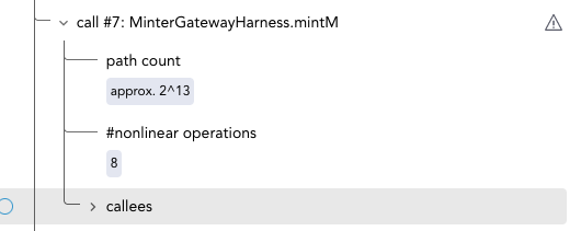
The Certora Prover indicates the path count in the Live Statistics panel. The path count is given once for the whole rule and separately on a per-call basis. The per-call path count always includes the paths of all deeper calls (the same holds for the count of nonlinear operations of the call).

Global and per-call path counts are displayed in the Live Statistics panel for each rule.

Path explosion

The number of paths given in the path count statistic might seem very high to users. The essential reason for these high numbers is known as the path explosion problem: The path count is usually exponential in the number of nodes and edges in the control flow graph.

For some intuition on how this happens, see the following illustration. Whenever there is a sequence of subgraphs that branch and then join again, the simplest variant of this being the diamond shapes in the picture, the path count of the whole graph is the product of these subgraph’s path counts. Thus, it is typical for the path count of a control flow graph to grow exponentially in its number of nodes (or edges).

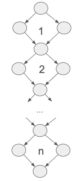
Illustration of path explosion through a sequence of n “diamond” shapes in the control flow graph. The shown control flow graph has 2ⁿ paths.

The path count statistic for a given rule is based on the control flow graph of the rule with all calls (and their calls and so forth) inlined. For example, if some method with 5 paths is called 10 times within the rule, its control flow graph will appear 10 times as a subgraph of the rule’s control flow graph. If, for instance, all these calls were made in sequence, and there was no further branching in the rule, the path count would be 5¹⁰.

For EVM, a particular potential cause for path explosion are DISPATCHER summaries. How much a DISPATCHER summary contributes to the path count depends on three factors:

• How many potential call targets are there (how many known implementations)

• How often the summarized function is called

• Whether the function is called in sequence or in parallel in the control flow (generally, control flow branchings in sequence lead to an exponential path explosion)

Mitigation approaches

To reduce the path count of a rule, the usual modularization techniques, like method summarization, can be applied. (See also the section Modular verification below.)

As pointed out in the previous sub-section, DISPATCHER summaries can lead to a path explosion, so replacing them, for instance, with AUTO summaries can have a significant impact. (See also AUTO summaries.)

Furthermore, it can help to change the parameters of the control flow splitting feature of the Certora Prover. Control flow splitting is a natural area to consider when the path count of a rule is high. When applying this technique, the Certora Prover internally divides each verification condition into smaller subproblems and attempts to solve them separately. For a more detailed explanation, see Control flow splitting.

We list a few option combinations that can help in various settings. There is a tradeoff between spending time in different places: The Prover can either try to spend much time at a low splitting level in the hope that no further splitting will be needed, or it can split quickly in the hope that the subproblems will be much easier to solve.

The options for control flow splitting are described in more detail in the corresponding section of the CLI documentation. In the following, we list some brief examples of how they can be used to avoid timeouts in certain scenarios.

When the relevant source code is very large, the shallow splits have a chance of being too large for the solvers, thus eager splitting might help:

certoraRun ... --prover_args '-smt_initialSplitDepth 5 -depth 15'

When there are very many subproblems medium difficulty, there is a chance that the Prover has to split too often (not being able to “close” any sub-splits). In that case, a lazier splitting strategy could help. We achieve lazier splitting by giving the solver more time to find a solution before we split a problem.

certoraRun ... --prover_args '-mediumTimeout 30 -depth 5'

It can also help to have splitting run in parallel (the splits are solved sequentially by default).

certoraRun ... --prover_args '-splitParallel true'

If the expectation is that the rule is violated (or not violated in case of a satisfy-style rule), the -dontStopAtFirstSplitTimeout option can prove useful.

certoraRun ... --prover_args '-dontStopAtFirstSplitTimeout true -depth 15 -mediumTimeout 5' --smt_timeout 10

Dealing with nonlinear arithmetic

Nonlinear integer arithmetic is often the hardest part of the formulas that the Certora Prover is solving.

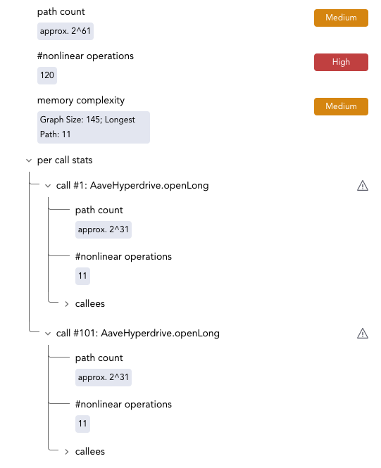
The Certora Prover displays the absolute number of nonlinear operations and their number per call in the Live Statistics panel. The per-call display has a warning sign next to the call when there is a non-trivial number of nonlinear operations in the call or its sub-call. Rules with two or more nonlinear operations are marked in this way.

For EVM, unless the detection of internal functions fails, both internal and external calls are considered in the statistics. If the detection fails (which should be rare), internal calls are treated as inlined into the external calls. In that case, each inlined internal call’s statistics contribute to the statistics of the enclosing external call.

Field in the Live Statistics panel indicating the number of nonlinear operations in the selected rule

Note

Counting the number of nonlinear operations is a rather coarse statistic. There are formulas with 10 nonlinear operations that are out of reach of current SMT solvers, while in other cases formulas with 120 operations are solved. Nevertheless, reducing the number of nonlinear operations has often proven a successful measure in timeout prevention, even if some remained.

The main techniques for reducing these numbers are modularization and underapproximation.

Modularization, typically by introducing method summaries, can help reduce the size of the rule, thus reducing the nonlinear operations. The per-call statistics in the Live Statistics panel (picture below) can help identify nonlinearity hot spots. Summarizing these hot spots, in particular, can help reduce the number of nonlinear operations, especially when a method is called multiple times.

Entry in Live Statistics indicating the number of operations are made in a given call, including its sub-calls

In some rules it is feasible to only consider an underapproximation of the actual behavior by fixing some value that is used very often in nonlinear computations to a concrete value. A typical example would be the decimal digits in fixed decimal arithmetic – having this unconstrained can increase nonlinearity in the rule massively, although only a small range of values is actually feasible. Of course, great care must be taken when choosing these underapproximations since they may lead to missed bugs.

A weaker form of underapproximation would be to introduce an extra requirement on the range of some variable that contributes to nonlinearity. For example, for the number of decimals in a fixed decimal computation, only values between 0 and 256 make sense, and in practice, values from an even smaller range are likely to be used. This measure will not change the values in the Live Statistics panel, but it has prevented timeouts in some cases nonetheless.

Dealing with high memory (or storage) complexity

Note

This section is EVM-specific and does not apply to Solana or Soroban.

The memory complexity of each rule or parametric rule is displayed in the Live Statistics panel in the Certora Prover reports.

The Certora Prover decompiles bytecode so that all EVM primitives can ultimately be modeled as SMT constructs. This process introduces key-to-value mappings for EVM memory and EVM storage. Additionally, the CVL specification may introduce ghost mappings. The Prover runs static analyses to reduce the load on these mappings by splitting them into smaller pieces (smaller mappings or scalar variables). However, this is not always possible, and some mappings usually remain in the final SMT formula.

Under this model, “memory updates” is a measure of how many times we store into a key-value mapping such as memory, storage, or a ghost function. The “longest update sequence” statistic represents the length the longest sequence of updates (i.e. store operations) performed on one of the mappings. In both cases, a smaller number indicates a less difficult problem for the Prover to solve.

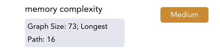
Entry in the Live Statistics panel indicating memory complexity

In the following we consider common culprits for high memory complexity.

Passing complex structs

One common reason for high memory complexity is complex data structures in the program or specification. struct types that contain many dynamically-sized arrays are especially problematic.

rule myRule() {
    MyStruct x;
    foo(x);

}

struct MyStruct {
    // several dynamically-sized arrays
    bytes b;
    string s;
    uint[] u1;
    uint8[] u2;
}

function foo(MyStruct x) public {
    ...
}

In this case, it can help to identify fields of the struct that are not relevant to the property of the program that is currently being reasoned about and comment out those fields. In our experience, these fields exist relatively often, especially in large structs. Naturally, the removal might be complicated because all usages of these fields also need some munging steps applied to them.

Memory and storage in inline assembly

The Certora Prover employs static analyses and simplifications to make reasoning about Storage and Memory easier for SMT solvers. However, unusual code patterns (most often produced when using inline assembly) can sometimes throw off these static analyses, making the SMT formulas too hard to solve.

CVT reports of Storage or Memory analysis failures in the Global Problems pane of the reports, along with pointers to the offending source code positions (typically inline assembly containing sstore/sload/mstore/mload operations). To resolve such failures, the relevant code parts need to be summarized or munged. (Naturally, the Certora developers are working to make such failures less frequent as well.)

Modular verification

Often, it is useful to break a complex problem into simpler subproblems; this process is called modularization. You can modularize a verification problem by first proving a property about a complex piece of code (such as a library or a method) and then using that property to summarize the complex code. In the following, we elaborate on modularization techniques that can help prevent timeouts.

Library-based systems

Note

This section is EVM-specific and does not apply to Solana or Soroban.

As mentioned here before, systems with libraries are a natural candidate for modularization.

As an alternative to using the -summarizeExtLibraryCallsAsNonDetPreLinking true option mentioned before, one can summarize all the methods of a single library using a catch-all summary. For example, to use a NONDET summary for all functions of MyBigLibrary, one could add the following:

methods {
    function MyBigLibrary._ external => NONDET;
    function MyBigLibrary._ internal => NONDET;
}

The above snippet has the effect of summarizing as NONDET all external calls to the library and internal ones as well. Only NONDET and HAVOC summaries can be applied. For more information on method summaries, see Summaries.

Command line options

There are several command line options that influence specific parts of the Prover’s pipeline. While their default values generally yield the best results, changing them can improve running time in certain cases.

--prover_args '-destructiveOptimizations enable'

This option enables some aggressive simplifications that speed up the Prover in many cases, but breaks call trace generation in case a rule is violated.